Quickstart

Estimating activities of fixed signatures

To inject fixed signature definitions into the probabilistic model, we use pymc3’s “observed variable” functionality. Once observed, the signature definitions will not be updated during inference.

[23]:

import pymc3 as pm
import arviz as az
import numpy as np
import pandas as pd
import damuta as da
import seaborn as sns
import matplotlib.pyplot as plt

[24]:

# Load data for 100 patients
counts = pd.read_csv('example_data/pcawg_counts.csv', index_col=0).head(100)
annotation = pd.read_csv('example_data/pcawg_cancer_types.csv', index_col=0).head(100)
pcawg = da.DataSet(counts, annotation)

To fix the damage signatures, we will observe phi. To fix the misrepair signatures, we will observe eta in the C context, and in the T context.

[25]:

damuta_sigs = da.SignatureSet.from_damage_misrepair(
    pd.read_csv('example_data/damage_signatures.csv', index_col=0),
    pd.read_csv('example_data/misrepair_signatures.csv', index_col=0))

[5]:

ht_lda = da.models.HierarchicalTandemLda(pcawg, type_col = 'pcawg_class',
                                         phi_obs= damuta_sigs.damage_signatures.to_numpy(),
                                         etaC_obs= damuta_sigs.misrepair_signatures[['C>A', 'C>G', 'C>T']].to_numpy(),
                                         etaT_obs= damuta_sigs.misrepair_signatures[['T>A', 'T>C', 'T>G']].to_numpy())

ht_lda._build_model(**ht_lda._model_kwargs)

[6]:

ht_lda.fit(n=10000)

100.00% [10000/10000 00:54<00:00 Average Loss = 4.642e+05]

Finished [100%]: Average Loss = 4.641e+05

[6]:

<damuta.models.HierarchicalTandemLda at 0x2b721300bf70>

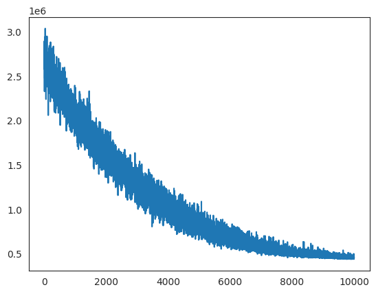
Check for nice convergence

[10]:

plt.plot(ht_lda.approx.hist)

[10]:

[<matplotlib.lines.Line2D at 0x2b723e9e7f40>]

Under the hood

Signature activities can be estimated from the product of the damage activities (\(\theta\)) and the association matrix (\(A\)). We call this product \(W\), where for draw \(d\) from the posterior, genome \(g\), damage signature \(i\) and misrepair signature \(j\), \(W_{dgij} = \theta_{dgi} A_{dgij}\). Because of the compositional properties of signature activities, \(\Sigma_{i}\theta_{dgi} = 1\) and \(\Sigma_{j}A_{dgij} = 1\). This means we can conveinently marginalize over the damage, and misrepair axes of \(W\) to get damage activities \(\theta_{dgi} = \Sigma_{j}W_{dgij}\) and misrepair activities \(\Gamma_{gdj} = \Sigma_{i}W_{dgij}\)

Let’s see this in code:

[11]:

trace = ht_lda.approx.sample(10)
trace

[11]:

<MultiTrace: 1 chains, 10 iterations, 17 variables>

[12]:

print("theta shape: ", trace.theta.shape)
print("A shape: ", trace.A.shape)

# reshape A for broadcasting
# nb. only necssary for hierarchical model
A = np.moveaxis(trace.A,1,2)
print("A reshaped: ", A.shape)

# compute W
W = (trace.theta[:,:,:,None]*A)
print("W shape: ", W.shape)

# check that W sums to theta over the misrepair axis
print("W correctly marginalizes to theta: ", np.allclose(W.sum(-1), trace.theta))

theta = W.sum(-1)
gamma = W.sum(-2)

# display mean over 10 posterior samples
display(pd.DataFrame(theta.mean(0)))
display(pd.DataFrame(gamma.mean(0)))

theta shape:  (10, 100, 18)
A shape:  (10, 18, 100, 6)
A reshaped:  (10, 100, 18, 6)
W shape:  (10, 100, 18, 6)
W correctly marginalizes to theta:  True

	0	1	2	3	4	5	6	7	8	9	10	11	12	13	14	15	16	17
0	0.018148	0.041422	0.014217	0.052663	0.049612	0.058811	0.071537	0.130497	0.066573	0.035261	0.021667	0.124121	0.016808	0.030907	0.047377	0.071972	0.010440	0.137968
1	0.196696	0.004420	0.018841	0.013270	0.016926	0.023671	0.162195	0.036593	0.076675	0.004726	0.011317	0.014630	0.046820	0.001704	0.091335	0.083935	0.110214	0.086030
2	0.027179	0.006244	0.020942	0.027659	0.007212	0.034248	0.241564	0.087762	0.029229	0.004069	0.006210	0.070710	0.011210	0.035043	0.059892	0.302042	0.011307	0.017476
3	0.162715	0.004495	0.024484	0.009229	0.004569	0.041733	0.107043	0.059714	0.041113	0.005306	0.005099	0.077870	0.032388	0.010351	0.045068	0.151163	0.194221	0.023440
4	0.048726	0.018671	0.032167	0.007728	0.022793	0.087195	0.101831	0.098192	0.027594	0.013096	0.010840	0.159202	0.026011	0.014519	0.140401	0.085658	0.087918	0.017457
...	...	...	...	...	...	...	...	...	...	...	...	...	...	...	...	...	...	...
95	0.023237	0.019154	0.055715	0.034148	0.021770	0.023628	0.105320	0.071424	0.036490	0.016433	0.017406	0.146123	0.033986	0.041399	0.088043	0.140026	0.047384	0.078316
96	0.093214	0.020699	0.045064	0.006078	0.028922	0.009975	0.060595	0.115997	0.037020	0.019665	0.025236	0.122353	0.013375	0.007978	0.087475	0.055401	0.183467	0.067485
97	0.076210	0.067483	0.022933	0.066986	0.074895	0.005201	0.042560	0.062713	0.028507	0.047743	0.024556	0.085347	0.026325	0.074539	0.064278	0.060788	0.119847	0.049088
98	0.003044	0.548510	0.011509	0.002059	0.162906	0.002314	0.001786	0.002327	0.002376	0.233313	0.011635	0.002660	0.001525	0.001529	0.004957	0.002173	0.003206	0.002169
99	0.005570	0.034685	0.004559	0.012614	0.019075	0.003656	0.007450	0.003930	0.007216	0.089470	0.504362	0.004362	0.238739	0.034096	0.004049	0.015485	0.006049	0.004633

100 rows × 18 columns

	0	1	2	3	4	5
0	0.119163	0.076473	0.033622	0.310843	0.269885	0.190014
1	0.140634	0.207480	0.173554	0.163602	0.179140	0.135590
2	0.054899	0.075041	0.357446	0.180587	0.311875	0.020151
3	0.145366	0.079770	0.395346	0.118004	0.064376	0.197138
4	0.169410	0.085609	0.276751	0.183347	0.103106	0.181778
...	...	...	...	...	...	...
95	0.096294	0.147463	0.156497	0.402184	0.147838	0.049724
96	0.195606	0.115633	0.135081	0.174319	0.179204	0.200157
97	0.144579	0.157569	0.080419	0.222177	0.083163	0.312092
98	0.039981	0.020032	0.152037	0.574859	0.018432	0.194659
99	0.014965	0.869613	0.036159	0.010102	0.051987	0.017174

100 rows × 6 columns

This functionality is implemented in the TandemLDA class as the convience method get_estimated_activities_DataFrame() which also adds back the sample index and turns it into a data frame. You could equally run this several times to get multiple posterior samples.

To get the estimated activities for the signatures we provided:

[13]:

theta_df, gamma_df = ht_lda.get_estimated_activities_DataFrame()
display(theta_df)
display(gamma_df)

	D1	D2	D3	D4	D5	D6	D7	D8	D9	D10	D11	D12	D13	D14	D15	D16	D17	D18
0009b464-b376-4fbc-8a56-da538269a02f	0.023905	0.042144	0.012821	0.067622	0.056636	0.052268	0.082317	0.125302	0.062317	0.015641	0.014897	0.094237	0.012628	0.026428	0.068918	0.082709	0.005059	0.154153
003819bc-c415-4e76-887c-931d60ed39e7	0.342639	0.000648	0.000514	0.006578	0.001124	0.028850	0.302648	0.020001	0.009185	0.001387	0.004508	0.002299	0.018233	0.000272	0.052665	0.128304	0.069978	0.010169
0040b1b6-b07a-4b6e-90ef-133523eaf412	0.023239	0.011639	0.034848	0.020823	0.007424	0.042319	0.187420	0.131227	0.031996	0.009143	0.002698	0.094749	0.015183	0.038535	0.138407	0.188625	0.009798	0.011924
00493087-9d9d-40ca-86d5-936f1b951c93	0.101447	0.008213	0.013212	0.010309	0.005631	0.054491	0.121498	0.051175	0.032020	0.009884	0.003356	0.122218	0.036383	0.009040	0.046290	0.121395	0.216920	0.036517
00508f2b-36bf-44fc-b66b-97e1f3e40bfa	0.076686	0.015870	0.031908	0.005782	0.053613	0.040126	0.136935	0.066822	0.037307	0.015242	0.006176	0.096585	0.024535	0.010237	0.201561	0.077706	0.076108	0.026801
...	...	...	...	...	...	...	...	...	...	...	...	...	...	...	...	...	...	...
09508a0d-ebe0-4fa1-b7b2-1710814181cd	0.014024	0.011455	0.042805	0.025631	0.024104	0.018295	0.159575	0.060968	0.041322	0.016498	0.014966	0.119394	0.034835	0.045682	0.144392	0.098213	0.044423	0.083417
09537dce-c797-4b60-962a-d4c3cd6ab00a	0.058662	0.027545	0.069911	0.006142	0.014077	0.013516	0.040982	0.075351	0.033984	0.012531	0.020908	0.086793	0.035255	0.010054	0.047830	0.056556	0.313982	0.075921
0972bfcf-c6c6-48cc-b820-cdfa6279a4f3	0.102685	0.088997	0.027429	0.055779	0.096025	0.006440	0.027940	0.047849	0.024664	0.042652	0.018933	0.084635	0.031575	0.085959	0.042514	0.057240	0.102292	0.056391
097a7d36-905b-72be-e050-11ac0d482c9a	0.002253	0.502181	0.007545	0.003651	0.146801	0.002077	0.002475	0.002219	0.003480	0.302682	0.007014	0.001481	0.001848	0.001913	0.004758	0.001927	0.002163	0.003533
0980e7fd-051d-45e9-9ca6-2baf073da4e8	0.007027	0.029439	0.003883	0.008763	0.010373	0.004535	0.012142	0.005621	0.005090	0.055001	0.486708	0.006488	0.287687	0.055831	0.004111	0.008387	0.005773	0.003141

100 rows × 18 columns

	M1	M2	M3	M4	M5	M6
0009b464-b376-4fbc-8a56-da538269a02f	0.216004	0.073933	0.029688	0.213874	0.283196	0.183304
003819bc-c415-4e76-887c-931d60ed39e7	0.106277	0.192278	0.297297	0.079554	0.190696	0.133898
0040b1b6-b07a-4b6e-90ef-133523eaf412	0.057356	0.082956	0.455159	0.125351	0.258156	0.021023
00493087-9d9d-40ca-86d5-936f1b951c93	0.116519	0.084419	0.374920	0.138902	0.057322	0.227917
00508f2b-36bf-44fc-b66b-97e1f3e40bfa	0.184631	0.112263	0.333812	0.143893	0.069998	0.155402
...	...	...	...	...	...	...
09508a0d-ebe0-4fa1-b7b2-1710814181cd	0.102007	0.172737	0.135884	0.403288	0.128281	0.057803
09537dce-c797-4b60-962a-d4c3cd6ab00a	0.221085	0.090471	0.089220	0.152718	0.224753	0.221753
0972bfcf-c6c6-48cc-b820-cdfa6279a4f3	0.140435	0.180135	0.082728	0.243320	0.092420	0.260961
097a7d36-905b-72be-e050-11ac0d482c9a	0.034730	0.015996	0.110241	0.587700	0.017674	0.233658
0980e7fd-051d-45e9-9ca6-2baf073da4e8	0.014682	0.856701	0.041231	0.010088	0.062320	0.014977

100 rows × 6 columns

The DAMUTA model classes wrap pymc3 - we just saw how to sample a MultiTrace from the posterior, and we can also turn this into arviz InferenceData

[14]:

idata = az.from_pymc3(trace, model = ht_lda.model)

[15]:

idata

[15]:

arviz.InferenceData

Visualizing uncertainty

We’ve stepped through several ways to get posterior samples. For most purposes, the get_estimated_activities_DataFrame() method is probably suitable to work with. However, it returns the mean of samples from the posterior, so when we want to make use of uncertainty estimates we should use the array equivalent: get_estimated_activities() which can return objects with >2 dimensions.

These objects are calculated as described above in “Under the hood” and dimensions correspond to n_draws x n_genomes x n_signatures

[16]:

theta, gamma = ht_lda.get_estimated_activities(n_draws = 10)

print("theta shape: ", theta.shape)
print("gamma shape: ", gamma.shape)

theta shape:  (10, 100, 18)
gamma shape:  (10, 100, 6)

Let’s look at just the first three patients. We can view the damage signature activity and the uncertainty, taking the mean and standard deviation of our 10 samples.

[17]:

patient_index = [0,1,2]
display(pcawg.annotation.iloc[patient_index])

	pcawg_class
guid
0009b464-b376-4fbc-8a56-da538269a02f	Ovary-AdenoCA
003819bc-c415-4e76-887c-931d60ed39e7	CNS-PiloAstro
0040b1b6-b07a-4b6e-90ef-133523eaf412	Liver-HCC

lets compile our theta and gamma samples into dataframes, for easy visualization

[18]:

theta_df = pd.concat([pd.DataFrame(theta[draw,patient_index,:],
              index = pcawg.annotation.iloc[patient_index].index,
              columns = ["D"+str(i+1) for i in range(ht_lda.n_damage_sigs)]).assign(posterior_sample = draw) for draw in range(10)])

theta_df['pcawg_class'] = pcawg.annotation.iloc[patient_index].pcawg_class
theta_df = theta_df.melt(id_vars = ['pcawg_class', 'posterior_sample'], var_name = 'Damage signature', value_name = 'theta')
theta_df.head()

[18]:

	pcawg_class	posterior_sample	Damage signature	theta
0	Ovary-AdenoCA	0	D1	0.022982
1	CNS-PiloAstro	0	D1	0.030673
2	Liver-HCC	0	D1	0.024449
3	Ovary-AdenoCA	1	D1	0.015198
4	CNS-PiloAstro	1	D1	0.047383

[19]:

gamma_df = pd.concat([pd.DataFrame(gamma[draw,patient_index,:],
              index =  pcawg.annotation.iloc[patient_index].index,
              columns = ["M"+str(i+1) for i in range(ht_lda.n_misrepair_sigs)]).assign(posterior_sample = draw) for draw in range(10)])
gamma_df['pcawg_class'] = pcawg.annotation.iloc[patient_index].pcawg_class
gamma_df = gamma_df.melt(id_vars = ['pcawg_class', 'posterior_sample'], var_name = 'Misrepair signature', value_name = 'gamma')
gamma_df.head()

[19]:

	pcawg_class	posterior_sample	Misrepair signature	gamma
0	Ovary-AdenoCA	0	M1	0.095974
1	CNS-PiloAstro	0	M1	0.133630
2	Liver-HCC	0	M1	0.037630
3	Ovary-AdenoCA	1	M1	0.108157
4	CNS-PiloAstro	1	M1	0.144083

Now plot the activities and uncertainty!

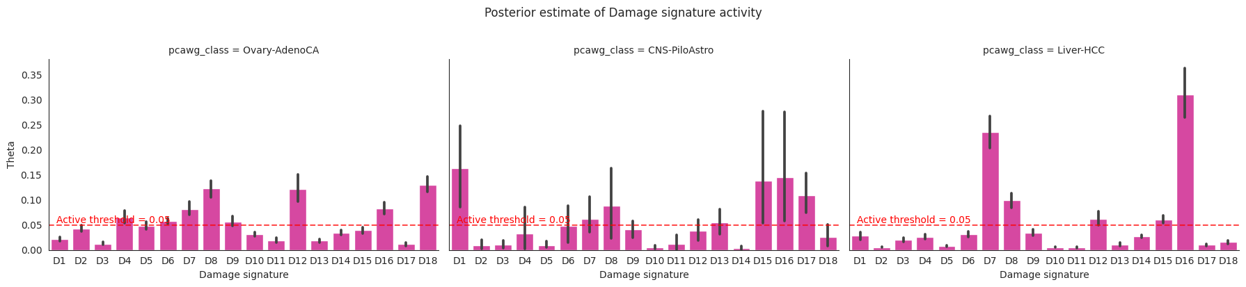
[20]:

g = sns.FacetGrid(theta_df, col='pcawg_class', col_wrap=3, height=4, aspect=1.5)
g.map_dataframe(sns.barplot, x='Damage signature', y='theta', color = '#EE30A7')
g.fig.suptitle('Posterior estimate of Damage signature activity', y=1.02)
g.set_axis_labels('Damage signature', 'Theta')
for ax in g.axes.flat:
    ax.text(2.5, 0.05, 'Active threshold = 0.05', ha='center', va='bottom', fontsize=10, color='red')
    ax.axhline(y=0.05, color='red', linestyle='--', alpha=0.7)
plt.tight_layout()
plt.show()

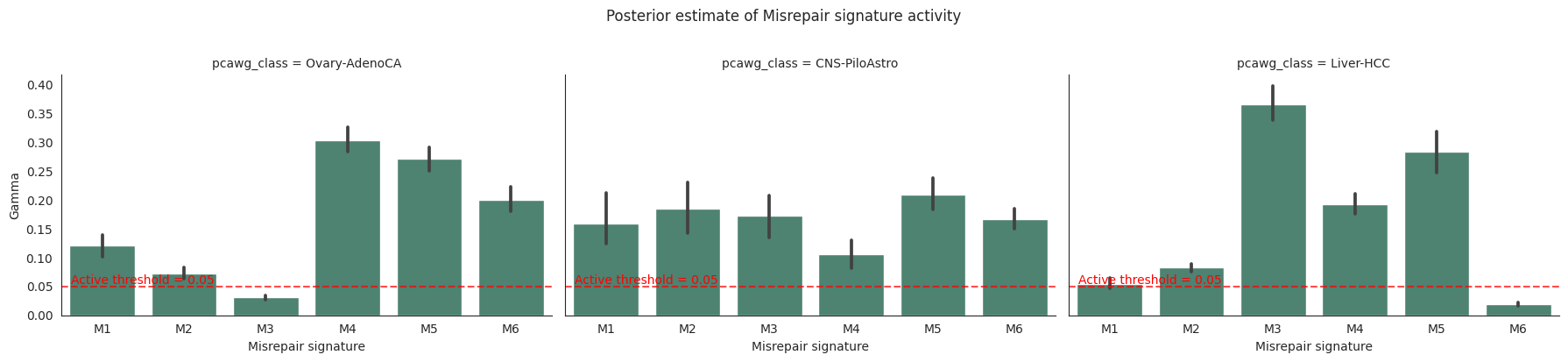
[21]:

g = sns.FacetGrid(gamma_df, col='pcawg_class', col_wrap=3, height=4, aspect=1.5)
g.map_dataframe(sns.barplot, x='Misrepair signature', y='gamma', color = '#458B74')
g.fig.suptitle('Posterior estimate of Misrepair signature activity', y=1.02)
g.set_axis_labels('Misrepair signature', 'Gamma')
for ax in g.axes.flat:
    ax.text(0.5, 0.05, 'Active threshold = 0.05', ha='center', va='bottom', fontsize=10, color='red')
    ax.axhline(y=0.05, color='red', linestyle='--', alpha=0.7)
plt.tight_layout()
plt.show()